Working with Excel: tutorial. Excel (Excel) is one of the basic programs of the package Microsoft Office. This is an indispensable assistant when working with invoices, reports, and tables.
Excel allows you to:
program, store huge amounts of information
Build graphs and analyze results
Make calculations quickly
This program is an excellent choice for office work.
Getting started with Excel (Excel)
1. Double-click on the sheet name to enter editing mode. In this panel, you can add a new sheet to the book or delete an unnecessary one. This is easy to do - you need to right-click and select the “Delete” line.
2. It’s easy to create another book - select the “Create” line in the “File” menu. The new book will be placed on top of the old one, and an additional tab will appear on the taskbar.

Working with tables and formulas
3. An important function of Excel is convenient work with tables.

Thanks to the tabular form of data presentation, tables automatically turn into a database. It is customary to format tables; to do this, select the cells and give them individual properties and format.

In the same window, you can perform alignment in a cell; this is done by the “Alignment” tab.

The Font tab has the option to change the font of text in a cell, and the Insert Menu allows you to add and remove columns, rows, and more.

Moving cells is easy - the “Cut” icon on the Home tab will help you with this.

4. No less important than the ability to work with tables is the skill of creating formulas and functions in Excel.

A simple F=ma is the formula, force equals mass times acceleration.

To write such a formula in Excel, you must start with the “=” sign.

Printing a document
5. And the main stage after the work is completed is printing the documents.
If you have read the previous ones, you should be aware that the formula begins with the “Equals” sign. When it becomes necessary to write this sign in a cell without a formula, the program persistently continues to consider such an entry as the beginning of the formula. When you click on another cell, the cell address is written after the sign. In this case, there are several ways to outsmart Excel.
An example of using the multiplication and equal signsSolution:
Place a space or an apostrophe before writing an equal sign, plus (addition), minus (subtraction), slash (division) or asterisk (multiplication).
Why doesn't the formula calculate in Excel?
If you have to work for different computers, then you may have to deal with the fact that necessary in the work Excel files They do not calculate using formulas.
Incorrect cell format or incorrect cell range settings
In Excel, various hashtag (#) errors occur, such as #VALUE!, #REF!, #NUMBER!, #N/A, #DIV/0!, #NAME? and #EMPTY!. They indicate that something in the formula is not working correctly. There may be several reasons.
Instead of the result it is given #VALUE!(in version 2010) or displays the formula in text format (in version 2016).
 Examples of errors in formulas
 In this example you can see that the contents of the cells are multiplied with different types data =C4*D4.
Bug fix: indicating the correct address =C4*E4 and copying the formula for the entire range.
- Error #LINK! Occurs when a formula references cells that have been deleted or replaced with other data.
- Error #NUMBER! Occurs when a formula or function contains an invalid numeric value.
- Error #N/A usually means that the formula does not find the requested value.
- Error #DIV/0! occurs when a number is divisible by zero (0).
- Error #NAME? occurs due to a typo in the formula name, that is, the formula contains a reference to a name that is not defined in Excel.
- Error #EMPTY! Occurs when an intersection is specified between two areas that do not actually intersect, or an incorrect separator is used between references when specifying a range.
Note:#### does not indicate a formula error, but rather that the column is not wide enough to display the contents of the cells. Simply drag the column border to expand it, or use the option Home - Format - Automatic column width selection.
Errors in formulas
Green triangles in the corner of a cell may indicate an error: numbers are written as text. Numbers stored as text may produce unexpected results.
Correction: Select a cell or range of cells. Click the "Error" sign (see picture) and select the desired action.
 An example of fixing errors in Excel
 Formula display mode enabled
Since in normal mode the calculated values are displayed in the cells, in order to directly see the calculated formulas in Excel there is a mode for displaying all formulas on the sheet. You can enable or disable this mode using the command Show formulas from tab Formulas in section Formula dependencies.
Automatic calculation using formulas is disabled
This is possible in files with a large amount of calculations. In order to weak computer did not slow down, the author of the file can disable automatic calculation in the file properties.
Correction: after changing the data, press the F9 button to update the results or enable automatic calculation. File – Options – Formulas – Calculation options – Calculations in the workbook: automatically.
Addition formula in Excel
Adding in spreadsheets is fairly easy. You need to write a formula that lists all the cells containing the data to be added. Of course, we put a plus between the cell addresses. For example, =C6+C7+C8+C9+C10+C11.
 Example of calculating a sum in Excel
 But if there are too many cells, then it is better to use the built-in function Autosum. To do this, click the cell in which the result will be displayed, and then click the button Autosum on the tab Formulas(highlighted with a red frame).
 Example of using the AutoSum function
 The range of cells to be summed will be highlighted. If the range was selected incorrectly, for example, vertical cells are selected, but horizontal ones are needed, then select a new range. To do this, left-click on the outermost cell of the new range and, without releasing the button, drag the pointer through all cells of the range to the final one. Complete the formula by pressing the key Enter on the keyboard.
Formula for rounding to a whole number in Excel
Beginner users use formatting that some try to round a number with. However, this does not affect the contents of the cell in any way, as indicated in the tooltip. When you click on the button (see figure), the format of the number will change, that is, its visible part will change, but the contents of the cell will remain unchanged. This can be seen in the formula bar.
 Decreasing bit depth does not round the number
 To round a number according to mathematical rules, you must use the built-in function =ROUND(number,number_of_digits).
 Mathematical rounding of a number using the built-in function
 You can write it manually or use the function wizard on the tab Formulas in the group Mathematical(see picture).
 Excel Function Wizard
 This function can round not only the fractional part of a number, but also whole numbers to the desired digit. To do this, when writing the formula, indicate the number of digits with a minus sign.
How to calculate percentages of a number
To calculate percentages in a spreadsheet, select the cell to enter the calculation formula. Place the equal sign, then write the address of the cell (use the English layout) that contains the number from which you will calculate the percentage. You can simply click on this cell and the address will be inserted automatically. Next, put the multiplication sign and enter the number of percentages that need to be calculated. Look at an example of calculating a discount when purchasing a product.
Formula =C4*(1-D4)
 Calculating the cost of a product taking into account the discount
 IN C4 the price of the vacuum cleaner is written down, and in D4– discount in %. It is necessary to calculate the cost of the product minus the discount; for this, our formula uses the construction (1-D4). Here the percentage value by which the price of the product is multiplied is calculated. For Excel, a record of the form 15% means the number 0.15, so it is subtracted from one. As a result, we get a residual value of the goods of 85% of the original.
In this simple way, using spreadsheets, you can quickly calculate percentages of any number.
Excel formula cheat sheet
The cheat sheet is made in the form of a PDF file. It includes the most popular formulas from the following categories: mathematical, text, logical, statistical. To get the cheat sheet, click the link below.
PS: Interesting facts about the real cost of popular goods
Dear reader! You have watched the article to the end.
Have you received an answer to your question? Write a few words in the comments.
If you haven't found the answer, indicate what you were looking for.
Microsoft Excel- it's convenient, multifunctional program, which is part of the Microsoft Office suite. The main purpose of the program is to compile tables, carry out calculations, systematize and analyze data, construct charts and graphs. Some people immediately have a question: “how to work in Excel?” Everything is very simple, to begin with, just learn the basic basic features, and then move on to more complex functions.
There are many professions for which the ability to work in xl makes it easier and faster to complete assigned tasks, for example: secretaries, managers, logisticians, accountants, economists, etc.
How excel works
In general, the work of this program can be characterized as a unified mathematical apparatus capable of performing various calculations based on given data and specified formulas.
To date, many versions of this program have been released. The latest is Microsoft Excel 2019. At the same time, the main specifics of the spreadsheet editor do not change, but are only improved. For example, in latest version added 6 new types of charts, functions FORECAST.ETS, CONCAT, IFS, MAXIFS, SWITCH, TEXTJOIN, updated joint editing mode, etc.
Excel interface
The Excel document itself consists of worksheets, each of which is a spreadsheet. They can be deleted, inserted, and named. The interface contains a large number of different elements: tabs, cells, various functions, built-in templates, etc.
Tab bar
This is a set of commands located on the horizontal ribbon at the top of the window. You can use the cursor to select the required section of the tab. For example, “Home” is responsible for the text in the document - font, location in a cell, formatting, etc.
Above the menu tabs in many versions of the program there is a panel quick access. Below the tab bar there is another line, consisting of two parts:
- The left side is called the cell name line. In Fig. 1 it says “R1C1” - this is the name of the cell, which is highlighted in black. It should be noted that many people change the reference style from four-digit (in this case “R1C1”) to two-digit. To do this, go to the “Excel Options” section and uncheck the box. In Fig. 2 you can see how to do this (highlighted in red) and what the result will be (highlighted in blue). Thanks to the cell name line, if there is a large amount of information, you can easily determine where the cursor is in the document.
- The right half is called the formula bar. In Fig. 1 - “fx” In this line you can see the contents of any cell; to do this, just “stand in the cell” with the cursor.
Cells
Tables can be filled with numerical values, text, date symbols, and formulas. The entered data is displayed in the formula bar, as described above, and in the cell itself in which the mouse cursor is positioned. Once you have completed your entry, you must press the Enter key on your keyboard to save the value in the desired location.
There are certain subtleties when entering decimal numbers, fractions, dates and times. As for the amount of text, the limitation is the cell width, but it can be increased. After entering the required information, you need to move the cursor between the column headers, double-click with the mouse, and the cell width will be automatically adjusted.
Formulas and functions
Before indicating the formula, you must put an equal sign. For example, we stand in the desired cell and indicate: “=8+9”, then press “Enter”, as a result in the cell we will see the number “17”, and in the formula line “fx” the action “=8+9”. You can use various mathematical operations: multiplication, division, subtraction, use parentheses.
In addition to numbers in the formula, you can specify cell numbers, then the data specified in them will participate in the mathematical operation. For example, in cell “A1” there is “4”, in “B1” - “3”, and in “C1” the formula is fixed: “=A1+B1”, as a result in cell “C1” the number “7” will appear, and in the formula line “fx” - action “=A1+B1” (Fig. 3).
A separate operation is provided for calculating summary totals. You need to “stand in the cell” in which the result should be displayed and click on the tab bar, in the “Home” section, the “ ” icon or the keyboard shortcut (ALT + =).
These are the easiest and simplest formulas; after studying them, you can move on to more complex calculations.
Excel has many different functions. A separate article should be dedicated to their description. If you are interested this topic, then if you wish, you can learn more in Excel courses https://spbshb.ru/secretarial-school/excel-courses. The simplest function that is most often used is the autocomplete marker. In order to use the marker, you need to select the desired cell, move the cursor to the lower right corner and wait for a thin black cross to appear.
After “dragging” it (with the left mouse button) over the required cells, the value following the previous one will be displayed in them. For example, the first cell contains the month “January”. After “dragging” the cursor in the corresponding cells the following will appear: “February, March, April”, etc. And if you need to specify the same value, then you additionally need to press the “Ctrl” key on the keyboard and you will get the required data in all the cells over which the cursor was “dragged”. You can also copy formulas.
Built-in templates
This program offers a wide variety of built-in templates for work: “account statement”, “personal budget”, etc. (Fig. 4). You can make changes and create your own templates.
To create charts and graphs, just select the necessary data from the completed table, select “Insert” in the tab bar and the “Histogram” tool, “Graph” - what needs to be generated, specify the desired form. The result will not keep you waiting long.
How to create a table in excel - basics
There are two ways:
- Fill in the cells, outline the borders of the table and save.
- In the tab bar, select “Insert” and the “Table” tool. In the information message that opens, specify the table range. Check the box for table with headers and click OK. The basis of the table is formed, you can enter data. If additional rows or columns are needed, just place the cursor in the desired cell, enter the data and press “Enter”. The table range will automatically expand. You can also use the autocomplete marker feature.
This entire article is only a partial description of how to work in xl. If you need to use complex calculations, linking to databases, you should turn to specialized literature or take courses, since the possibilities Microsoft programs Excel is big.
Anyone who uses a computer in their daily work has, in one way or another, encountered the Excel office application, which is part of the standard Microsoft Office package. It is available in any version of the package. And quite often, when starting to get acquainted with the program, many users wonder whether they can use Excel on their own?
What is Excel?
First, let's define what Excel is and what this application is needed for. Many people have probably heard that the program is a spreadsheet editor, but the principles of its operation are fundamentally different from the same tables created in Word.
If in Word a table is more of an element in which a text or table is displayed, then a sheet with an Excel table is, in fact, a unified mathematical machine that is capable of performing a wide variety of calculations based on specified data types and formulas by which this or that mathematical or algebraic operation.
How to learn to work in Excel on your own and is it possible to do it?
As the heroine of the film “Office Romance” said, you can teach a hare to smoke. In principle, nothing is impossible. Let's try to understand the basic principles of the application's functioning and focus on understanding its main capabilities.
Of course, reviews from people who understand the specifics of the application say that you can, say, download some tutorial on working in Excel, however, as practice shows, and especially comments from novice users, such materials are very often presented in a too abstruse form, and It can be quite difficult to figure out.
It seems that the best training option would be to study the basic capabilities of the program, and then apply them, so to speak, “by scientific poking.” It goes without saying that you first need to consider the basic functional elements of Microsoft Excel (the program lessons indicate exactly this) in order to get a complete picture of the principles of operation.
Key elements to pay attention to
The very first thing the user pays attention to when launching the application is a sheet in the form of a table, in which cells are located, numbered in different ways, depending on the version of the application itself. IN earlier versions Columns were designated by letters, and rows by numbers and numbers. In other releases, all markings are presented exclusively in digital form.

What is this for? Yes, only so that it is always possible to determine the cell number for specifying a certain calculation operation, similar to how coordinates are specified in a two-dimensional system for a point. Later it will be clear how to work with them.
Another important component is the formula bar - a special field with an “f x” icon on the left. This is where all operations are specified. At the same time, the mathematical operations themselves are designated in exactly the same way as is customary in the international classification (equal sign “=”, multiplication “*” division “/”, etc.). Trigonometric quantities also correspond to international notations (sin, cos, tg, etc.). But this is the simplest thing. More complex operations will have to be mastered with the help of the help system or specific examples, since some formulas may look quite specific (exponential, logarithmic, tensor, matrix, etc.).
Above, as in others office programs there is a main panel and main menu sections with main operation points and quick access buttons to a particular function.
and simple operations with them
Consideration of the question is impossible without a key understanding of the types of data entered in table cells. Let us immediately note that after entering some information, you can press the enter button, the Esc key, or simply move the rectangle from the desired cell to another - the data will be saved. Editing a cell is done by double-clicking or pressing the F2 key, and upon completion of data entry, saving occurs only by pressing the Enter key.

Now a few words about what can be entered in each cell. The format menu is called up by right-clicking on active cell. On the left there is a special column indicating the data type (general, numeric, text, percentage, date, etc.). If the general format is selected, the program, roughly speaking, itself determines what exactly the entered value looks like (for example, if you enter 01/01/16, the date January 1, 2016 will be recognized).

When entering a number, you can also use an indication of the number of decimal places (by default, one character is displayed, although when entering two, the program simply rounds the visible value, although the true value does not change).
When using, say, a text data type, whatever the user types will be displayed exactly as typed on the keyboard, without modification.
Here's what's interesting: if you hover the cursor over the selected cell, a cross will appear in the lower right corner, by pulling it while holding down the left mouse button, you can copy the data to the cells following the desired one in order. But the data will change. If we take the same date example, the next value would be January 2, and so on. This type of copying can be useful when specifying the same formula for different cells (sometimes even with cross calculations).
When it comes to formulas, for the simplest operations you can use a two-pronged approach. For example, for the sum of cells A1 and B1, which must be calculated in cell C1, you need to place the rectangle in the C1 field and specify the calculation using the formula “=A1+B1”. You can do it differently by setting the equality “=SUM(A1:B1)” (this method is more used for large gaps between cells, although you can use the automatic sum function, as well as the English version of the SUM command).
Excel program: how to work with Excel sheets
When working with sheets, you can perform many actions: add sheets, change their name, delete unnecessary ones, etc. But the most important thing is that any cells located on different sheets can be interconnected certain formulas(especially when large amounts of information of different types are entered).

How to learn to work in Excel on your own in terms of use and calculations? It's not that simple here. As reviews from users who have mastered this spreadsheet editor show, it will be quite difficult to do this without outside help. You should at least read the help system of the program itself. The simplest way is to enter cells in the same formula by selecting them (this can be done both on one sheet and on different ones. Again, if you enter the sum of several fields, you can enter “=SUM”, and then simply select one by one while holding down the Ctrl key the necessary cells. But this is the most primitive example.
Additional features
But in the program you can not only create tables with various types data. Based on them, in a couple of seconds you can build all kinds of graphs and diagrams by specifying either a selected range of cells for automatic construction, or specifying it in manual mode when entering the corresponding menu.

In addition, the program has the ability to use special add-ons and executable scripts based on Visual Basic. You can insert any objects in the form of graphics, video, audio or anything else. In general, there are enough opportunities. And here only a small fraction of everything that this unique program is capable of is touched upon.
What can I say, with the right approach it can calculate matrices, solve all kinds of equations of any complexity, find, create databases and link them with other applications like Microsoft Access and much more - you just can’t list them all.
Bottom line
Now, it’s probably already clear that the question of how to learn to work in Excel on your own is not so easy to consider. Of course, if you master the basic principles of working in the editor, setting the simplest operations will not be difficult. User reviews indicate that you can learn this in a maximum of a week. But if you need to use more complex calculations, and even more so, work with reference to databases, no matter how much anyone wants it, you simply cannot do without special literature or courses. Moreover, it is very likely that you will even have to improve your knowledge of algebra and geometry from the school course. Without this, you can’t even dream of fully using the spreadsheet editor.
Microsoft Excel is convenient for creating tables and making calculations. A workspace is a set of cells that can be filled with data. Subsequently – format, use for building graphs, charts, summary reports.
Working with Excel tables for novice users may seem difficult at first glance. It differs significantly from the principles of creating tables in Word. But we'll start small: by creating and formatting a table. And at the end of the article, you will already understand that you cannot imagine a better tool for creating tables than Excel.
How to Create a Table in Excel for Dummies
Working with tables in Excel for dummies is not rushed. You can create a table in different ways and for specific purposes, each method has its own advantages. Therefore, first let’s visually assess the situation.
Take a close look at the spreadsheet worksheet:
This is a set of cells in columns and rows. Essentially a table. Columns are indicated in Latin letters. Lines are numbers. If we print this sheet, we will get a blank page. Without any boundaries.
First let's learn how to work with cells, rows and columns.
How to select a column and row
To select the entire column, click on its name (Latin letter) with the left mouse button.

To select a line, use the line name (by number).

To select several columns or rows, left-click on the name, hold and drag.
To select a column using hot keys, place the cursor in any cell of the desired column - press Ctrl + spacebar. To select a line – Shift + spacebar.
How to change cell borders
If the information does not fit when filling out the table, you need to change the cell borders:


To change the width of columns and height of rows at once in a certain range, select an area, increase 1 column/row (move manually) - the size of all selected columns and rows will automatically change.

Note. To return to the previous size, you can click the “Cancel” button or the CTRL+Z hotkey combination. But it works when you do it right away. Later it won't help.
To return the lines to their original boundaries, open the tool menu: “Home” - “Format” and select “Auto-fit line height”

This method is not relevant for columns. Click “Format” - “Default Width”. Let's remember this number. Select any cell in the column whose borders need to be “returned”. Again “Format” - “Column Width” - enter specified by the program indicator (usually 8.43 - the number of characters in the Calibri font with a size of 11 points). OK.
How to insert a column or row
Select the column/row to the right/below the place where you want to insert the new range. That is, the column will appear to the left of the selected cell. And the line is higher.

Right-click and select “Insert” from the drop-down menu (or press the hotkey combination CTRL+SHIFT+"=").

Mark the “column” and click OK.
Advice. To quickly insert a column, select the column in the desired location and press CTRL+SHIFT+"=".
All these skills will come in handy when creating a table in Excel. We will have to expand the boundaries, add rows/columns as we work.
Step-by-step creation of a table with formulas


Column and row borders will now be visible when printing.

Using the Font menu, you can format Excel table data as you would in Word.

Change, for example, the font size, make the header “bold”. You can center the text, assign hyphens, etc.
How to create a table in Excel: step-by-step instructions
The simplest way to create tables is already known. But Excel has a more convenient option (in terms of subsequent formatting and working with data).
Let's make a “smart” (dynamic) table:

Note. You can take a different path - first select a range of cells, and then click the “Table” button.

Now enter the necessary data into the finished frame. If you need an additional column, place the cursor in the cell designated for the name. Enter the name and press ENTER. The range will automatically expand.

If you need to increase the number of lines, hook it in the lower right corner to the autofill marker and drag it down.
How to work with a table in Excel
With the release of new versions of the program, working with tables in Excel has become more interesting and dynamic. When a smart table is formed on a sheet, the “Working with Tables” - “Design” tool becomes available.
Here we can give the table a name and change its size.
Various styles are available, the ability to convert the table into a regular range or a summary report.
Features of dynamic MS Excel spreadsheets huge. Let's start with basic data entry and autofill skills:


If we click on the arrow to the right of each header subheading, we will get access to additional tools for working with table data.

Sometimes the user has to work with huge tables. To see the results, you need to scroll through more than one thousand lines. Deleting rows is not an option (the data will be needed later). But you can hide it. For this purpose, use numerical filters (picture above). Uncheck the boxes next to the values that should be hidden.